Nominal T Method
In Nominal T model of Transmission line, the whole shunt capacitance of line is assumed to be lumped at the middle of the line. The half of the line resistance and reactance is assumed at either side of the shunt capacitance as shown in figure below. Due to such modeling of line, capacitive charging current is flowing through half of the transmission line. Mind that, this is not the case in End Condenser method. In End Condenser method, capacitive charging current flows through the entire line as shunt capacitance is assumed to be lumped at the receiving end.

Let us now try to find the sending end voltage and current. For that, we will apply kirchhof’s law. Each parameter is shown in figure above with their meaning.
As the voltage across the shunt capacitance
V1 = (R/2 + jX/2)IR + VR ………(1)
Also, using Kirchhof’s current law,
Is = IR + Ic (phasor sum) ………………………….(2)
Therefore,
Vs = (R/2 + jX/2)Is + V1
= (R/2 + jX/2)IR + (R/2 + jX/2)Is + VR …………………….(3)
Let us now take the receiving end voltage as reference and assume that receiving end current or load current is lagging by some angle ØR.
Therefore,
VR = VR + j0
and IR = IR<-ØR = IR (CosØR – jSinØR)
As the current through the shunt capacitor lead by an angle 90° with respect to voltage across it i.e. V1, therefore
Ic = jωCV1
From equation (2),
Is = IR (CosØR – jSinØR) + jωCV1
= IR CosØR + j(ωCV1 – SinØR) ………………..(4)
Thus by putting the value of V1 from equation (1) in equation (4), sending end current can be found. Similarly, the sending end voltage can be calculated by putting the value of Is in equation (3). Voltage Regulation can also be calculated as we know the sending and receiving end voltage.
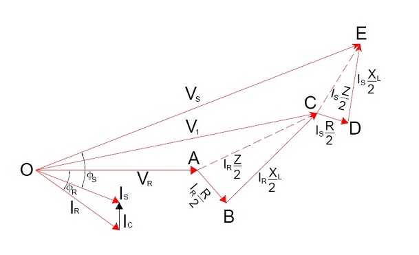
See, I haven’t used phasor diagram to find these parameters. The phasor diagram for Nominal T method is shown below.
Nominal π Method
In Nominal π Method, the shunt capacitance of each line i.e. phase to neutral is divided into two equal parts. One part is lumped at the sending end while the other is lumped at receiving end as shown in figure below.
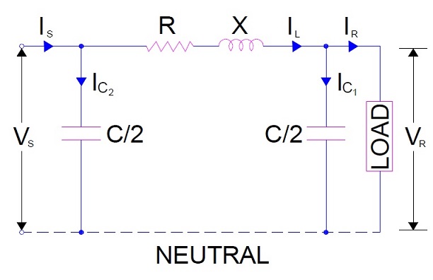
Notice that, in this method there is no effect of shunt capacitance at sending end on the line voltage drop and hence on voltage regulation but this accounts for the charging current in sending end.
Let
IR = Load Current per phase
R = Resistance per phase
X = Reactance per phase
C = Capacitance per phase
CosØR = Receiving end power factor (lagging)
Vs = Sending end voltage
Let us now draw the phasor. Assume receiving end voltage VR as reference and load current IR lagging this voltage by ØR.
Therefore,
VR = VR + j0
and IR = IR<-ØR = IR (CosØR – jSinØR)
Charging Current at load end IC1 = j(ωC/2)VR = jπfCVR
Line Current IL = IR + IC1 (phasor sum)
Sending end voltage Vs = VR + IL (R+jX)
Now,
Charging current at sending end IC2 = j(ωC/2)Vs = jπfCVs
Hence, Sending end current Is = IL + IC2 (phasor sum)
Thus sending end current and voltage is calculated as above and from these parameters the performance of line is evaluated.
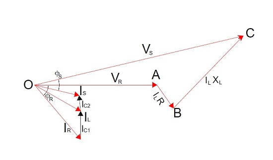
Can u please give the phasor diagram for nominal pi?
Please refer the second phasor diagram in the post, it is the phasor diagram of nominal pi model.
Can you please draw the phasor diagram of a leading power factor
Can you please draw the phasor diagram of a leading power factor